
Using the following example, we will explore the various functions of the power applet:
Suppose that an educational testing company created a training program named “ACE” to help students improve their scores on a standardized exam. The company spokesman boasts that ACE graduates score higher on a standardized test than the population of individuals who do not participate in their training course.
The WISE Power Applet (which is shown below as a static picture) will be used to simulate drawing a sample of graduates from the ACE program. At the top (Area A), the blue curve represents the population distribution for non-graduates (Null Population) while the red curve represents graduates from the ACE program (Alternative Population). For this exercise we assume both populations are normal distributions.
In the textboxes to the right (Area D), we can set values for the two population means (μ0 and μ1) and the population standard deviation (σ) by entering values into the textboxes. We can also set the number of cases to be sampled (n) and our alpha error rate (α). After changing any of these values, be sure to press Enter.
Pressing the Sample button (Area C) simulates drawing a sample of size n from the Alternative Population. The sample of n cases is shown as small yellow boxes in Area A and the sample mean is shown with a red arrow. The sample mean is also shown below relative to the two theoretical sampling distributions (Area B).
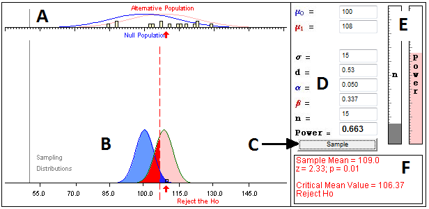
The dashed red line shows where we have set our alpha criterion. In this case we set α = .05, corresponding to the upper 5% of the blue null sampling distribution. If our sample mean is to the right of the dashed line, we can reject the null hypothesis with p < .05, one-tailed (and correctly conclude that the sample did not come from the null population). If a sample mean falls to the left of the dashed line, we fail to reject the null hypothesis. This would be a Type II or β error (i.e., failing to reject a false null hypothesis) because the sample was actually drawn from the alternate distribution.
The decision box (Area F) shows the sample mean and the z-value of the sample mean on the null distribution as well as the one-tailed p-value and the decision: Reject or do not reject the null hypothesis (H0). The z-score computed on the null sampling distribution allows us to determine the probability of observing a sample mean this large or larger if the null hypothesis is true. In the example shown here, the sample mean is 109.0 and the z-value on the null sampling distribution of the mean (blue) is 2.33. The probability of finding a z-score greater than 2.33 if we are sampling from the null distribution is p = 0.01. Because this probability is less than alpha (i.e., .05), our statistical decision is to reject H0.
Area D shows many statistical values including power and effect size, and Area E represents sample size (n) and power as ‘thermometers.’ In the actual applet on the next page you will be able to change any of these values.
![]()