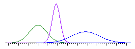
The normal distribution is defined by a mathematical formula. Although normal distributions may have different means and standard deviations, all normal distributions are “bell-curve” shaped, symmetrical with the greatest height at the mean (see Figure 1 for examples). Tails of a normal distribution are asymptotic, indefinitely decreasing but never touching the x-axis. The total area under the curve sums to 100%.

Figure 1. Three normal distributions whose means and standard deviations differ.
If we have a normal distribution, we can use the formula to calculate how likely it is to observe values in regions of interest.
Some measurements in the natural world may approximate normal distributions (e.g., perhaps the weights of hippopotamuses, heights of palm trees, students’ IQs, and people’s happiness). However, natural distributions are rarely (never?) exactly normal, or even close enough to normal that we can apply the formula with confidence.
A major reason why the normal distribution is so important in inferential statistics is because the distribution of possible sample means approaches normal as the sample size increases, as described by the Central Limit Theorem. This allows us to compute the probability of obtaining a sample mean in any range of interest, given that the sample is drawn randomly from a population with a specified mean and standard deviation.
Important note: Before we use the normal distribution to compute probabilities, we must verify that the distribution of interest is very close to normal. Although a distribution of scores in a sample of N cases may be quite far from normal, the distribution of means for all possible samples of N cases (i.e., the sampling distribution of the mean) may be quite close to normal. This fact, as described in the Central Limit Theorem, is critical for many applications of statistical inference.
Standard Normal Distributions and Z Scores
A normal distribution that is standardized (so that it has a mean of 0 and a S.D. of 1) is called the standard normal distribution, which represents a distribution of z-scores. If we know the mean μ (“mu”), and standard deviation σ (“sigma”), of a set of scores which are normally distributed, we can standardized each “raw” score, x, by converting it into a z score by using the following formula on each individual score:
![]()
A z score reflects how many standard deviations above or below the population mean a raw score is. For instance, on a scale which has a mean of 500 and a standard deviation of 100, a score of 450 would equal a z score of (450-500)/100 = -50/100 = -0.50, which indicates that the score is half a standard deviation below the mean.
- Note that converting x scores to z scores does NOT change the shape of the distribution. The distribution of z scores is normal if and only if the distribution of x is normal.
- Depending upon the sample size and the shape of the population distribution for x, the sampling distribution of means may be very close to a normal distribution even when the population distribution is not normal.
By converting normally distributed scores (either the observed data or the theoretical sampling distribution of the mean) into z scores, we can ascertain the probabilities of obtaining specific ranges of scores using either a table for the standard normal distribution (i.e., a z table) or a calculator like the WISE p-z converter.
Caution: It is not appropriate to use a normal distribution calculator or table to find probabilities unless you are confident that the shape of your distribution of interest is very close to the normal distribution!
Calculating a Z Score and Probability
Suppose that SAT scores among U.S. college students are normally distributed with a mean of 500 and a standard deviation of 100. What is the probability that a randomly selected individual from this population has an SAT score at or below 600?
Solve this yourself now. You may use either a z table of probabilities or the p–z converter to find the desired probability.
Hint: A correction for continuity is appropriate here.
Use the ‘back’ arrow on your browser to return to where your were.
![]()

