
The previous questions lead us to two important implications of the Central Limit Theorem. Compared to its parent (population) distribution, a sampling distribution has:
- the same mean, but
- a smaller variance.
Since samples contain many scores, extreme scores tend to cancel each other out and leave you with a pretty middle-of-the-road mean. So, when all these means are put in a sampling distribution there are very few means out in the extremes – the means tend to pile up around the middle. This is especially true when the sample size is large.
Below we’ve superimposed the sampling distribution of means for N = 81 over the population distribution. As you can see, the sampling distribution of the means is very skinny and very tall compared to the population distribution. Notice the relative probability of an observation of 5′ 7″ in each of these distributions. If we selected one woman at random from the population (where SD = 3), we would not be very surprised if her height was 5′ 7″. That height is only one standard deviation above the mean, so it is not very unusual.
However, if we took a random sample of N = 81 women and found the average height to be 5′ 7″, we would be very surprised. The distribution of means is much less variable, so a mean height of 5′ 7″ is extremely unlikely. A sample mean of 5′ 7″ represents a z-score of z = 9.00 (or a score that is nine standard deviations above the mean) on the sampling distribution of means, an extremely unlikely score on a normal distribution.
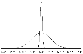
Figure. Sampling distribution of means, N = 81, superimposed over population distribution.
Why is z = 9.00 for 5′ 7″ when N = 81?
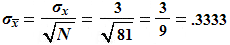
The standard error of the mean is equal to the population standard deviation, 3, divided by the square root of the sample size:
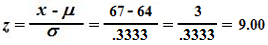
To calculate z, we subtract the mean (64 inches) from 5 feet, 7 inches (67 inches) and then divide by the standard error of the mean:
![]()